Multilinear Regression

by IndiaSuccessStories April 9, 2024

written by IndiaSuccessStories April 9, 2024

Multilinear Regression

Introduction

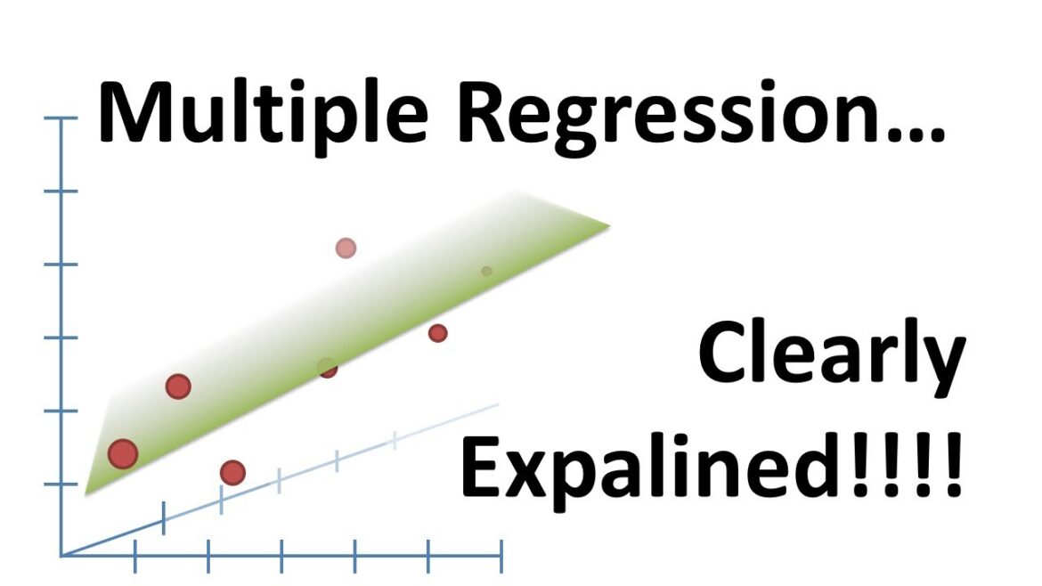
Multiple linear regression is an extension of simple linear regression that allows for the modeling of the relationship between multiple independent variables and a single dependent variable. In other words, it enables us to predict a continuous outcome based on two or more predictor variables.

Here's how it works and how to implement it:

How it works:

Model Representation

In multiple linear regression, the relationship between the independent variables X1,X2,...,Xn and the dependent variable y is represented by the equation:

y=β0+β1⋅X1+β2⋅X2+...+βn⋅Xn+ϵ

y is the dependent variable (the variable we want to predict).
X1,X2,...,Xn are the independent variables (features).
β0 is the intercept .
β1,β2,...,βn are the coefficients .
ϵ is the error term .

Objective

The objective is to estimate the coefficients β0,β1,...,βn that minimize the difference between the observed and predicted values of the dependent variable.

Model Training

We use a dataset with observations for both the independent variables and the dependent variable. The model is trained using techniques like ordinary least squares (OLS) to find the best-fitting line through the data.

Model Evaluation

After training, the model's performance is evaluated using metrics such as mean squared error (MSE), R-squared, or others, to assess how well the model fits the data and how much variance it explains.

Implementation

Import Libraries

import numpy as np

import pandas as pd

from sklearn.model_selection import train_test_split

from sklearn.linear_model import LinearRegression

from sklearn.metrics import mean_squared_error, r2_score

# Step 1: Collect Data

data = pd.read_csv('energy_efficiency.csv')

# Step 2: Explore the Data (omitted for brevity)

# Step 3: Data Preprocessing

X = data[['Relative_Compactness', 'Surface_Area', 'Wall_Area', 'Roof_Area', 'Overall_Height',

'Orientation', 'Glazing_Area', 'Glazing_Area_Distribution']] # Independent variables

y = data[['Heating_Load', 'Cooling_Load']] # Dependent variables

# Step 4: Split Data

X_train, X_test, y_train, y_test = train_test_split(X, y, test_size=0.2, random_state=42)

# Step 5: Create and Fit the Model

model = LinearRegression()

model.fit(X_train, y_train)

# Step 6: Make Predictions

y_pred = model.predict(X_test)

# Step 7: Evaluate the Model

mse = mean_squared_error(y_test, y_pred)

r_squared = r2_score(y_test, y_pred)

print("Mean Squared Error:", mse)

print("R-squared:", r_squared)

# Step 8: Interpret the Coefficients

coefficients = pd.DataFrame({'Variable': X.columns, 'Heating_Load_Coefficient': model.coef_[0],

'Cooling_Load_Coeff

IndiaSuccessStories

Indian Success Stories is committed to inspiring the world’s visionary leaders who are driven to make a difference with their ground-breaking concepts, ventures, and viewpoints. Join together with us to match your business with a community that is unstoppable and working to improve everyone’s future.

Multilinear Regression

Multilinear Regression

Introduction

Here's how it works and how to implement it:

How it works:

Implementation

Linear Regression

Polynomial Regression

You may also like

Leave a Comment Cancel Reply