Logistic Regression

Table of Contents

Logistic Regression

Introduction

Logistic Regression is a classification algorithm used to model the probability of a binary outcome based on one or more predictor variables. Despite its name, logistic regression is used for classification, not regression.

Here's how logistic regression works:

Here, z is the linear combination of the input features and their corresponding coefficients

Linear Combination

Similar to linear regression, logistic regression calculates a linear combination of the input features and their corresponding coefficients:

z=β0+β1x1+β2x2+…+βnxn

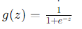
The linear combination z is then passed through the sigmoid function to obtain the predicted probability

Decision Boundary

Logistic regression predicts the probability that an observation belongs to a particular class (e.g., 0 or 1). By default, if the predicted probability is greater than or equal to 0.5, the observation is classified as belonging to class 1; otherwise, it's classified as belonging to class 0.
The decision boundary is the threshold value (usually 0.5) that separates the two classes.

Training

The logistic regression model is trained using maximum likelihood estimation. The goal is to find the coefficients β0,β1,…,βn that maximize the likelihood of observing the actual classes given the input features
This is typically done using optimization algorithms such as gradient descent or Newton's method

Evaluation

Once trained, the logistic regression model can be used to make predictions on new data points. Predictions are obtained by applying the trained model to the input features and converting the output probabilities into class labels using the decision boundary.

Regularization

Logistic regression can be regularized to prevent overfitting by adding penalty terms to the cost function. The two most common types of regularization are L1 regularization (Lasso) and L2 regularization (Ridge)

Interpretation

The coefficients β0,β1,…,βn of logistic regression provide insights into the relationship between the input features and the log-odds of the outcome. Positive coefficients indicate that an increase in the corresponding feature increases the probability of belonging to class 1, while negative coefficients indicate the opposite.

Logistic regression is widely used in various fields such as healthcare (predicting disease risk), marketing (customer churn prediction), and finance (credit risk assessment). It's a simple yet powerful algorithm for binary classification tasks.

Here's an example of logistic regression using the LogisticRegression class from scikit-learn:

We import the necessary libraries and modules from scikit-learn.

import numpy as np

import pandas as pd

import matplotlib.pyplot as plt

from sklearn.datasets import make_classification

from sklearn.model_selection import train_test_split

from sklearn.linear_model import LogisticRegression

from sklearn.metrics import accuracy_score, confusion_matrix, classification_report

We generate synthetic data using the make_classification function from scikit-learn. This function creates a random binary classification problem with a specified number of samples, features, and classes.

X, y = make_classification(n_samples=1000, n_features=2, n_classes=2, random_state=42)

We split the data into training and testing sets using the train_test_split

X_train, X_test, y_train, y_test = train_test_split(X, y, test_size=0.2, random_state=42)

We create an instance of the LogisticRegression class and fit it to the training data.

model = LogisticRegression()

model.fit(X_train, y_train)

We make predictions on the test data using the predict

y_pred = model.predict(X_test)

We evaluate the model's performance using metrics such as accuracy, confusion matrix, and classification report.

accuracy = accuracy_score(y_test, y_pred)

conf_matrix = confusion_matrix(y_test, y_pred)

class_report = classification_report(y_test, y_pred)

print("Accuracy:", accuracy)

print("Confusion Matrix:\n", conf_matrix)

print("Classification Report:\n", class_report)

Finally, we visualize the decision boundary of the logistic regression model using a scatter plot. The decision boundary separates the two classes based on the learned coefficients.

plt.figure(figsize=(10, 6))

plt.scatter(X[:, 0], X[:, 1], c=y, cmap='bwr', marker='o', alpha=0.6, label='Actual')

plt.xlabel('Feature 1')

plt.ylabel('Feature 2')

plt.title('Logistic Regression: Decision Boundary')

plt.legend()

plt.show()

This example demonstrates how to use logistic regression for a binary classification task. You can adjust hyperparameters like regularization strength (C), penalty (penalty), and solver (solver) to control the model's behavior and optimize its performance

Logistic Regression

Introduction

Here's how logistic regression works:

Here's an example of logistic regression using the LogisticRegression class from scikit-learn:

Useful Links

Edtior's Picks

Latest Articles

Logistic Regression

Logistic Regression

Introduction

Here's how logistic regression works:

Here's an example of logistic regression using the LogisticRegression class from scikit-learn:

Random Forest Regression

k-Nearest Neighbors (k-NN)

You may also like

Leave a Comment Cancel Reply

Useful Links

Edtior's Picks

Latest Articles