k-Nearest Neighbors (k-NN)
Introduction
k-Nearest Neighbors (k-NN) is a non-parametric and lazy learning algorithm used for both classification and regression tasks. It’s based on the idea that data points with similar features tend to belong to the same class or have similar target values.
Here's how k-Nearest Neighbors works:
- Data Representation
Each data point in the dataset is represented as a point in a multi-dimensional feature space, where each dimension corresponds to a feature or attribute
- Distance Metric
k-NN relies on a distance metric (e.g., Euclidean distance, Manhattan distance) to measure the similarity between data points in the feature space. The choice of distance metric depends on the nature of the data and the problem at hand.
- k-Nearest Neighbors
Given a new data point, the algorithm identifies the k nearest neighbors to that point based on the chosen distance metric. These neighbors are the data points with the smallest distances to the new point.
- Classification
For classification tasks, the algorithm assigns the majority class among the k nearest neighbors to the new data point. The class label of the new point is determined by a majority vote among its neighbors.
- Regression
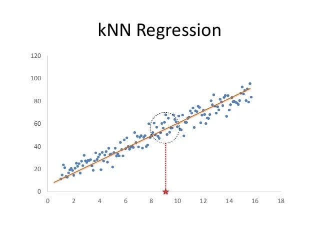
For regression tasks, the algorithm predicts the target value of the new data point by averaging the target values of its k nearest neighbors.
- Hyperparameter Tuning K
The number of neighbors k is a hyperparameter that needs to be specified by the user. Choosing the right value of k is crucial and can significantly impact the performance of the algorithm. A smaller value of k can lead to a more flexible model with higher variance but lower bias, while a larger value of k can lead to a smoother decision boundary with lower variance but higher bias.
- Scaling
It's important to scale the features before applying k-NN to avoid biased distances due to differences in feature scales.
- Computational Complexity
The main drawback of k-NN is its computational complexity during prediction, as it requires calculating distances to all training points. This makes it inefficient for large datasets with many dimensions.
- Curse of Dimensionality
In high-dimensional feature spaces, the concept of proximity becomes less meaningful, and the performance of k-NN can deteriorate due to the curse of dimensionality.
Despite its simplicity, k-NN can be effective for a wide range of classification and regression tasks, especially for small to medium-sized datasets with low dimensionality. However, its performance can degrade significantly in high-dimensional spaces or when dealing with imbalanced datasets.
Here's an example of how to use k-Nearest Neighbors (k-NN) for classification using the KNeighborsClassifier class from scikit-learn:
- We import the necessary libraries and modules from scikit-learn.
import numpy as np
import pandas as pd
import matplotlib.pyplot as plt
from sklearn.datasets import make_classification
from sklearn.model_selection import train_test_split
from sklearn.neighbors import KNeighborsClassifier
from sklearn.metrics import accuracy_score, confusion_matrix, classification_report
- We generate synthetic data using the make_classification function from scikit-learn. This function creates a random binary classification problem with a specified number of samples, features, and classes.
X, y = make_classification(n_samples=1000, n_features=2, n_classes=2, random_state=42)
- We split the data into training and testing sets using the train_test_split
X_train, X_test, y_train, y_test = train_test_split(X, y, test_size=0.2, random_state=42)
- We create an instance of the KNeighborsClassifier class with n_neighbors=5 (5 nearest neighbors) and fit it to the training data.
model = KNeighborsClassifier(n_neighbors=5)
model.fit(X_train, y_train)
- We make predictions on the test data using the predict
y_pred = model.predict(X_test)
- We evaluate the model's performance using metrics such as accuracy, confusion matrix, and classification report.
accuracy = accuracy_score(y_test, y_pred)
conf_matrix = confusion_matrix(y_test, y_pred)
class_report = classification_report(y_test, y_pred)
print("Accuracy:", accuracy)
print("Confusion Matrix:\n", conf_matrix)
print("Classification Report:\n", class_report)
- Finally, we visualize the decision boundary of the k-NN classifier using a scatter plot. The decision boundary separates the two classes based on the majority class of the nearest neighbors.
plt.figure(figsize=(10, 6))
plt.scatter(X[:, 0], X[:, 1], c=y, cmap='bwr', marker='o', alpha=0.6, label='Actual')
plt.xlabel('Feature 1')
plt.ylabel('Feature 2')
plt.title('k-Nearest Neighbors: Decision Boundary')
plt.legend()
plt.show()
This example demonstrates how to use k-Nearest Neighbors for a binary classification task. You can adjust the hyperparameter n_neighbors to control the number of neighbors considered during classification and optimize the model's performance.

