Support Vector Classification
Introduction
Support Vector Machines (SVM) are primarily used for classification tasks. However, there is a variant of SVM called Support Vector Regression (SVR) that is specifically designed for regression tasks. SVR aims to fit a function that approximates the relationship between the input features and the target variable in a continuous manner.
Here's how Support Vector Regression works:
- Margin
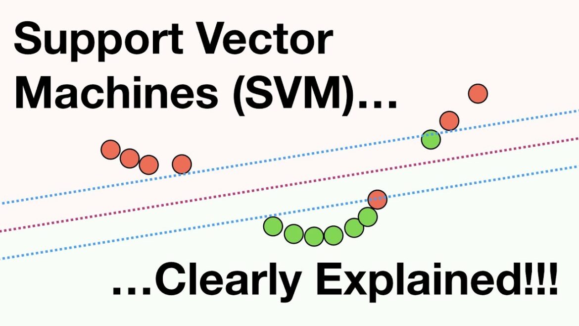
Similar to SVM for classification, SVR aims to find a hyperplane that maximizes the margin between the data points and the hyperplane while minimizing the margin violations. However, in SVR, the goal is to fit the hyperplane as closely as possible to the training data, rather than separating different classes.
- Epsilon-Insensitive Loss Function
SVR introduces an epsilon-insensitive loss function, which allows some errors to be ignored within a certain margin (epsilon). Data points within this margin are considered to have been correctly predicted and do not contribute to the loss.
- Support Vectors
The data points that lie on the margin or within the margin boundaries are called support vectors. These support vectors play a crucial role in determining the SVR model.
- Kernel Trick
SVR can utilize kernel functions (e.g., linear, polynomial, radial basis function) to map the input features into a higher-dimensional space. This allows SVR to capture non-linear relationships between the features and the target variable.
- Regularization Parameter(C)
Similar to SVM, SVR has a regularization parameter (C) that controls the trade-off between maximizing the margin and minimizing the error. A smaller C value allows for a wider margin but may lead to more training errors, while a larger C value reduces training errors but may lead to overfitting.
- Prediction
Once the SVR model is trained, it can be used to make predictions on new data points. The predicted values are obtained by evaluating the fitted function at the input feature values.
Support Vector Regression is useful for regression tasks, especially when dealing with non-linear relationships between the features and the target variable. By adjusting hyperparameters such as the choice of kernel function, epsilon, and regularization parameter, SVR can be fine-tuned to achieve optimal performance for different types of datasets.
Here's an example of how to use Support Vector Regression (SVR) for a regression task using the SVR class from scikit-learn in Python:
- We import the necessary libraries and modules from scikit-learn.
import numpy as np
import pandas as pd
import matplotlib.pyplot as plt
from sklearn.datasets import make_regression
from sklearn.model_selection import train_test_split
from sklearn.svm import SVR
from sklearn.metrics import mean_squared_error, r2_score
- We generate synthetic data using the make_regression function from scikit-learn. This function creates a random regression problem with a specified number of samples, features, noise, and random state.
X, y = make_regression(n_samples=1000, n_features=1, noise=20, random_state=42)
- We split the data into training and testing sets using the train_test_split
X_train, X_test, y_train, y_test = train_test_split(X, y, test_size=0.2, random_state=42)
- We create an instance of the SVR class with a radial basis function (RBF) kernel, regularization parameter C=100, and epsilon parameter epsilon=0.1, and fit it to the training data.
model = SVR(kernel='rbf', C=100, epsilon=0.1)
model.fit(X_train, y_train)
- We make predictions on the test data using the predict
y_pred = model.predict(X_test)
- We evaluate the model's performance using mean squared error (MSE) and R-squared.
mse = mean_squared_error(y_test, y_pred)
r2 = r2_score(y_test, y_pred)
print("Mean Squared Error:", mse)
print("R-squared:", r2)
- Finally, we visualize the actual versus predicted values using a scatter plot.
plt.figure(figsize=(10, 6))
plt.scatter(X_test, y_test, color='blue', label='Actual')
plt.scatter(X_test, y_pred, color='red', label='Predicted')
plt.xlabel('Feature')
plt.ylabel('Target')
plt.title('Support Vector Regression')
plt.legend()
plt.show()
This example demonstrates how to use Support Vector Regression for a regression task. You can adjust hyperparameters like the choice of kernel, regularization parameter C, and epsilon parameter epsilon to control the model's behavior and optimize its performance for different datasets

